This is a dataset of wine quality containing 4898 observations of 12 variables. The variables are:
fixed.acidity: The amount of fixed acid in the wine (\(g/dm^3\))
volatile.acidity: The amount of volatile acid in the wine (\(g/dm^4\))
citric.acid: The amount of citric acid in the wine (\(g/dm^3\))
residual.sugar: The amount of residual sugar in the wine (\(g/dm^3\))
chlorides: The amount of salt in the wine (\(g/dm^3\))
free.sulfur.dioxide: The amount of free sulfur dioxide in the wine (\(mg/dm^3\))
total.sulfur.dioxide: The amount of total sulfur dioxide in the wine (\(mg/dm^3\))
density: The density of the wine (\(g/dm^3\))
pH: The \(pH\) value of the wine
sulphates: The amount of sulphates in the wine (\(g/dm^3\))
alcohol: The alcohol content of the wine (\(\% vol\))
quality: The quality score of the wine (0-10)
After removing the duplicate rows from our data set, we are left with 3961 observations of the above 11 variables minus quality column variable, and introduced a new variable good as our response:
good: A binary variable indicating whether the wine is good (quality\(\geq\) 7) or not (quality\(<\) 7).
Data Import
Show/Hide Code
# Import original datasetwine.data <-read.csv("dataset\\winequality-white.csv", sep=";", header = T)str(wine.data)
 fixed.acidity    volatile.acidity  citric.acid     residual.sugar
 Min.   : 3.800   Min.   :0.0800   Min.   :0.0000   Min.   : 0.600
 1st Qu.: 6.300   1st Qu.:0.2100   1st Qu.:0.2700   1st Qu.: 1.700
 Median : 6.800   Median :0.2600   Median :0.3200   Median : 5.200
 Mean   : 6.855   Mean   :0.2782   Mean   :0.3342   Mean   : 6.391
 3rd Qu.: 7.300   3rd Qu.:0.3200   3rd Qu.:0.3900   3rd Qu.: 9.900
 Max.   :14.200   Max.   :1.1000   Max.   :1.6600   Max.   :65.800
   chlorides       free.sulfur.dioxide total.sulfur.dioxide    density
 Min.   :0.00900   Min.   :  2.00      Min.   :  9.0        Min.   :0.9871
 1st Qu.:0.03600   1st Qu.: 23.00      1st Qu.:108.0        1st Qu.:0.9917
 Median :0.04300   Median : 34.00      Median :134.0        Median :0.9937
 Mean   :0.04577   Mean   : 35.31      Mean   :138.4        Mean   :0.9940
 3rd Qu.:0.05000   3rd Qu.: 46.00      3rd Qu.:167.0        3rd Qu.:0.9961
 Max.   :0.34600   Max.   :289.00      Max.   :440.0        Max.   :1.0390
       pH          sulphates         alcohol         quality
 Min.   :2.720   Min.   :0.2200   Min.   : 8.00   Min.   :3.000
 1st Qu.:3.090   1st Qu.:0.4100   1st Qu.: 9.50   1st Qu.:5.000
 Median :3.180   Median :0.4700   Median :10.40   Median :6.000
 Mean   :3.188   Mean   :0.4898   Mean   :10.51   Mean   :5.878
 3rd Qu.:3.280   3rd Qu.:0.5500   3rd Qu.:11.40   3rd Qu.:6.000
 Max.   :3.820   Max.   :1.0800   Max.   :14.20   Max.   :9.000
Show/Hide Code
summary(wine.data_cleaned)
 fixed.acidity    volatile.acidity  citric.acid     residual.sugar
 Min.   : 3.800   Min.   :0.0800   Min.   :0.0000   Min.   : 0.600
 1st Qu.: 6.300   1st Qu.:0.2100   1st Qu.:0.2700   1st Qu.: 1.600
 Median : 6.800   Median :0.2600   Median :0.3200   Median : 4.700
 Mean   : 6.839   Mean   :0.2805   Mean   :0.3343   Mean   : 5.915
 3rd Qu.: 7.300   3rd Qu.:0.3300   3rd Qu.:0.3900   3rd Qu.: 8.900
 Max.   :14.200   Max.   :1.1000   Max.   :1.6600   Max.   :65.800
   chlorides       free.sulfur.dioxide total.sulfur.dioxide    density
 Min.   :0.00900   Min.   :  2.00      Min.   :  9.0        Min.   :0.9871
 1st Qu.:0.03500   1st Qu.: 23.00      1st Qu.:106.0        1st Qu.:0.9916
 Median :0.04200   Median : 33.00      Median :133.0        Median :0.9935
 Mean   :0.04591   Mean   : 34.89      Mean   :137.2        Mean   :0.9938
 3rd Qu.:0.05000   3rd Qu.: 45.00      3rd Qu.:166.0        3rd Qu.:0.9957
 Max.   :0.34600   Max.   :289.00      Max.   :440.0        Max.   :1.0390
       pH          sulphates         alcohol           good
 Min.   :2.720   Min.   :0.2200   Min.   : 8.00   Min.   :0.0000
 1st Qu.:3.090   1st Qu.:0.4100   1st Qu.: 9.50   1st Qu.:0.0000
 Median :3.180   Median :0.4800   Median :10.40   Median :0.0000
 Mean   :3.195   Mean   :0.4904   Mean   :10.59   Mean   :0.2083
 3rd Qu.:3.290   3rd Qu.:0.5500   3rd Qu.:11.40   3rd Qu.:0.0000
 Max.   :3.820   Max.   :1.0800   Max.   :14.20   Max.   :1.0000
Show/Hide Code
# Check for NAs in datasetsum(is.na(wine.data))
[1] 0
Show/Hide Code
# Counts for response's at each factor leveltable(wine.data$quality)
   3    4    5    6    7    8    9
  20  163 1457 2198  880  175    5
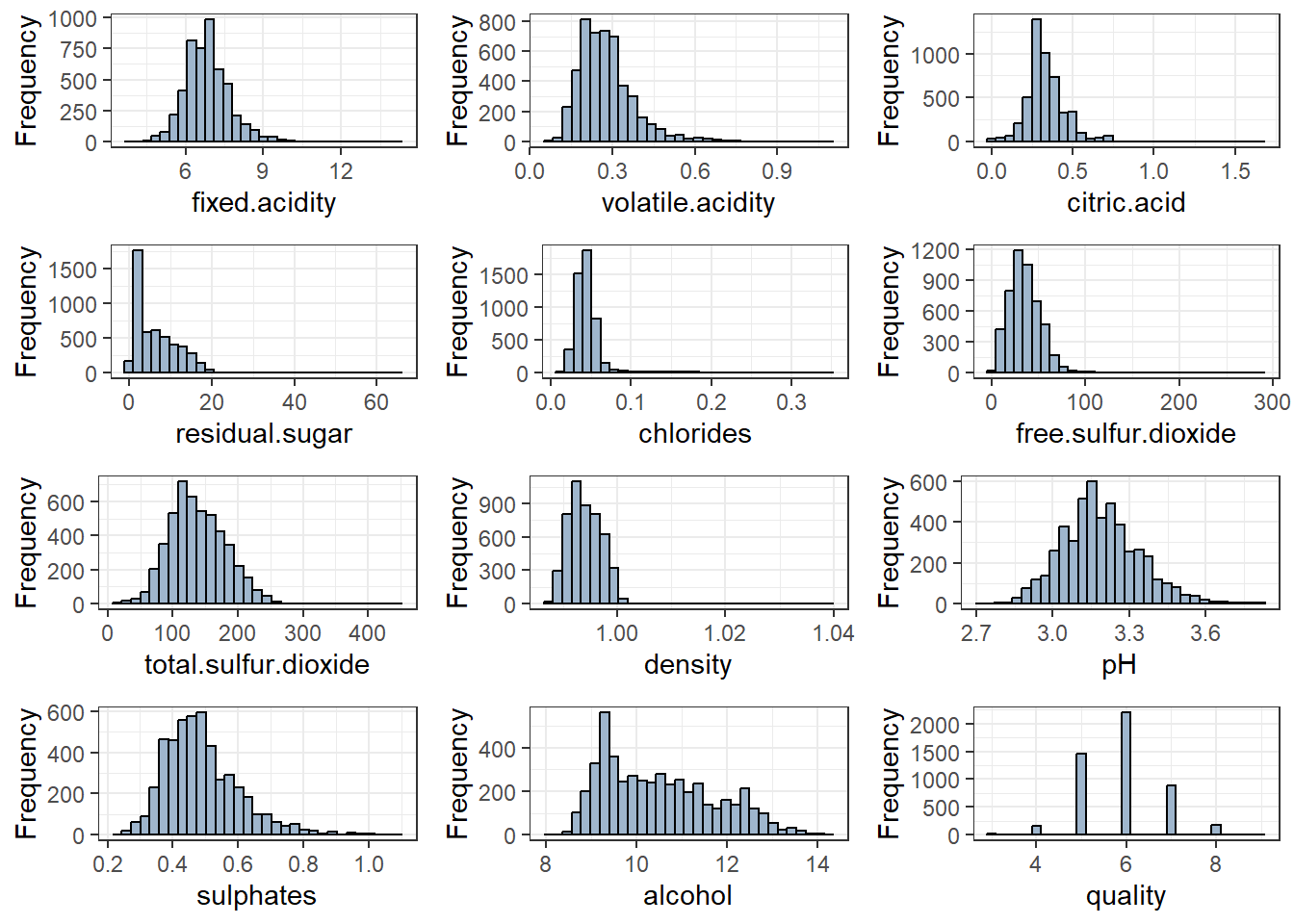
Data Distribution
Show/Hide Code
wine.colnames <-colnames(wine.data)num_plots <-length(wine.colnames)num_rows <-ceiling(num_plots/3)# Create an empty list to store plotsgrid_arr <-list()# Loop over each column name in the wine.colnames vectorfor(i in1:num_plots) {# Create a ggplot object for the current column using aes plt <-ggplot(data = wine.data, aes_string(x = wine.colnames[i])) +geom_histogram(binwidth =diff(range(wine.data[[wine.colnames[i]]]))/30, color ="black", fill ="slategray3") +labs(x = wine.colnames[i], y ="Frequency") +theme_bw()# Add the current plot to the grid_arr list grid_arr[[i]] <- plt}grid_arr <-do.call(gridExtra::grid.arrange, c(grid_arr, ncol =3))
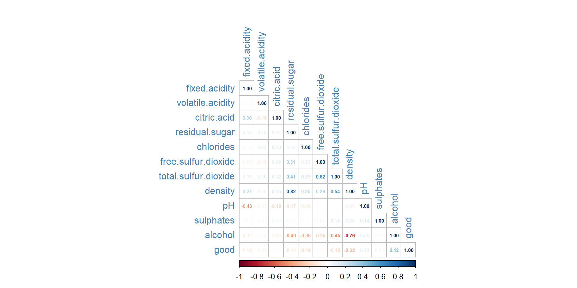
# Collinearity between Attributescor(wine.data_cleaned) %>% corrplot::corrplot(method ='number', type ="lower", tl.col ="steelblue", number.cex =0.5)
Data Split
Show/Hide Code
set.seed(1234)# Splitting the dataset into train and test (7/10th for train remaining for test)inTrain <- caret::createDataPartition(wine.data_cleaned$good, p =7/10, list = F)train <- wine.data_cleaned[inTrain,]test <- wine.data_cleaned[-inTrain,]# Convert the outcome variable to a factor with two levelstrain$good <-as.factor(train$good)test$good <-as.factor(test$good)# Save data for building models in the next stepsave(wine.data, file ="dataset\\wine.data.Rdata")save(wine.data_cleaned, file ="dataset\\wine.data_cleaned.Rdata")save(train, file ="dataset\\train.Rdata")save(test, file ="dataset\\test.Rdata")
Source Code
---title: "Exploratory Analysis"---```{r setup, include=FALSE}knitr::opts_chunk$set(fig.align =TRUE)library(tidyverse) # Load core packages: # ggplot2, for data visualization.# dplyr, for data manipulation.# tidyr, for data tidying.# purrr, for functional programming.# tibble, for tibbles, a modern re-imagining of data frames.# stringr, for strings.# forcats, for factors.# lubridate, for date/times.# readr, for reading .csv, .tsv, and .fwf files.# readxl, for reading .xls, and .xlxs files.# feather, for sharing with Python and other languages.# haven, for SPSS, SAS and Stata files.# httr, for web apis.# jsonlite for JSON.# rvest, for web scraping.# xml2, for XML.# modelr, for modelling within a pipeline# broom, for turning models into tidy data# hms, for times.library(magrittr) # Pipeline operatorlibrary(lobstr) # Visualizing abstract syntax trees, stack trees, and object sizeslibrary(pander) # Exporting/converting complex pandoc documents, EX: df to Pandoc tablelibrary(ggforce) # More plot functions on top of ggplot2library(ggpubr) # Automatically add p-values and significance levels plots. # Arrange and annotate multiple plots on the same page. # Change graphical parameters such as colors and labels.library(sf) # Geo-spatial vector manipulation: points, lines, polygonslibrary(kableExtra) # Generate 90 % of complex/advanced/self-customized/beautiful tableslibrary(cowplot) # Multiple plots arrangementlibrary(gridExtra) # Multiple plots arrangementlibrary(animation) # Animated figure containerlibrary(latex2exp) # Latex axis titles in ggplot2library(ellipse) # Simultaneous confidence interval region to check C.I. of 2 slope parameterslibrary(plotly) # User interactive plotslibrary(ellipse) # Simultaneous confidence interval region to check C.I. of 2 regressorslibrary(olsrr) # Model selections library(leaps) # Regression subsetting library(pls) # Partial Least squareslibrary(MASS) # LDA, QDA, OLS, Ridge Regression, Box-Cox, stepAIC, etc,.library(e1071) # Naive Bayesian Classfier,SVM, GKNN, ICA, LCAlibrary(class) # KNN, SOM, LVQlibrary(ROCR) # Precision/Recall/Sensitivity/Specificity performance plot library(boot) # LOOCV, Bootstrap,library(caret) # Classification/Regression Training, run ?caret::trainControllibrary(corrgram) # for correlation matrixlibrary(corrplot) # for graphical display of correlation matrixset.seed(1234) # make random results reproduciblecurrent_dir <-getwd()if (!is.null(current_dir)) {setwd(current_dir)remove(current_dir)}```## Data DescriptionThis is a dataset of wine quality containing 4898 observations of 12 variables. The variables are:- `fixed.acidity`: The amount of fixed acid in the wine ($g/dm^3$)- `volatile.acidity`: The amount of volatile acid in the wine ($g/dm^4$)- `citric.acid`: The amount of citric acid in the wine ($g/dm^3$)- `residual.sugar`: The amount of residual sugar in the wine ($g/dm^3$)- `chlorides`: The amount of salt in the wine ($g/dm^3$)- `free.sulfur.dioxide`: The amount of free sulfur dioxide in the wine ($mg/dm^3$)- `total.sulfur.dioxide`: The amount of total sulfur dioxide in the wine ($mg/dm^3$)- `density`: The density of the wine ($g/dm^3$)- `pH`: The $pH$ value of the wine- `sulphates`: The amount of sulphates in the wine ($g/dm^3$)- `alcohol`: The alcohol content of the wine ($\% vol$)- `quality`: The quality score of the wine (0-10)After removing the duplicate rows from our data set, we are left with 3961 observations of the above 11 variables minus `quality` column variable, and introduced a new variable `good` as our response:- `good`: A binary variable indicating whether the wine is good (`quality` $\geq$ 7) or not (`quality` $<$ 7).## Data Import```{r data_import}# Import original datasetwine.data <-read.csv("dataset\\winequality-white.csv", sep=";", header = T)str(wine.data)# Removing duplicate Rows, mutate our categorical response goodwine.data_cleaned <- wine.data %>%mutate(good =ifelse(quality>=7, 1, 0)) %>%distinct() %>% dplyr::select(-quality)str(wine.data_cleaned)```## Data Analysis```{r basic_analysis}dim(wine.data)dim(wine.data_cleaned)summary(wine.data)summary(wine.data_cleaned)# Check for NAs in datasetsum(is.na(wine.data))# Counts for response's at each factor leveltable(wine.data$quality)```## Data Distribution```{r hist_plot, warning=FALSE}wine.colnames <-colnames(wine.data)num_plots <-length(wine.colnames)num_rows <-ceiling(num_plots/3)# Create an empty list to store plotsgrid_arr <-list()# Loop over each column name in the wine.colnames vectorfor(i in1:num_plots) {# Create a ggplot object for the current column using aes plt <-ggplot(data = wine.data, aes_string(x = wine.colnames[i])) +geom_histogram(binwidth =diff(range(wine.data[[wine.colnames[i]]]))/30, color ="black", fill ="slategray3") +labs(x = wine.colnames[i], y ="Frequency") +theme_bw()# Add the current plot to the grid_arr list grid_arr[[i]] <- plt}grid_arr <-do.call(gridExtra::grid.arrange, c(grid_arr, ncol =3))``````{r, echo=FALSE}# Remove unnecessary variablesremove(grid_arr)remove(plt)remove(i)remove(num_plots)remove(num_rows)```## Data Relationships```{r relation_plot_original, fig.width=10, fig.height=5, message=FALSE}reshape2::melt(wine.data[, 1:12], "quality") %>%ggplot(aes(value, quality, color = variable)) +geom_point() +geom_smooth(aes(value, quality, colour=variable), method=lm, se=FALSE)+facet_wrap(.~variable, scales ="free")# Collinearity between Attributescor(wine.data) %>% corrplot::corrplot(method ='number', type ="lower", tl.col ="steelblue", number.cex =0.5)``````{r relation_plot_cleaned, fig.width=10, fig.height=5, message=FALSE}reshape2::melt(wine.data_cleaned[, 1:12], "good") %>%ggplot(aes(value, good, color = variable)) +geom_point() +geom_smooth(aes(value, good, colour=variable), method=lm, se=FALSE)+facet_wrap(.~variable, scales ="free")# Collinearity between Attributescor(wine.data_cleaned) %>% corrplot::corrplot(method ='number', type ="lower", tl.col ="steelblue", number.cex =0.5)```## Data Split```{r data_split}set.seed(1234)# Splitting the dataset into train and test (7/10th for train remaining for test)inTrain <- caret::createDataPartition(wine.data_cleaned$good, p =7/10, list = F)train <- wine.data_cleaned[inTrain,]test <- wine.data_cleaned[-inTrain,]# Convert the outcome variable to a factor with two levelstrain$good <-as.factor(train$good)test$good <-as.factor(test$good)# Save data for building models in the next stepsave(wine.data, file ="dataset\\wine.data.Rdata")save(wine.data_cleaned, file ="dataset\\wine.data_cleaned.Rdata")save(train, file ="dataset\\train.Rdata")save(test, file ="dataset\\test.Rdata")```