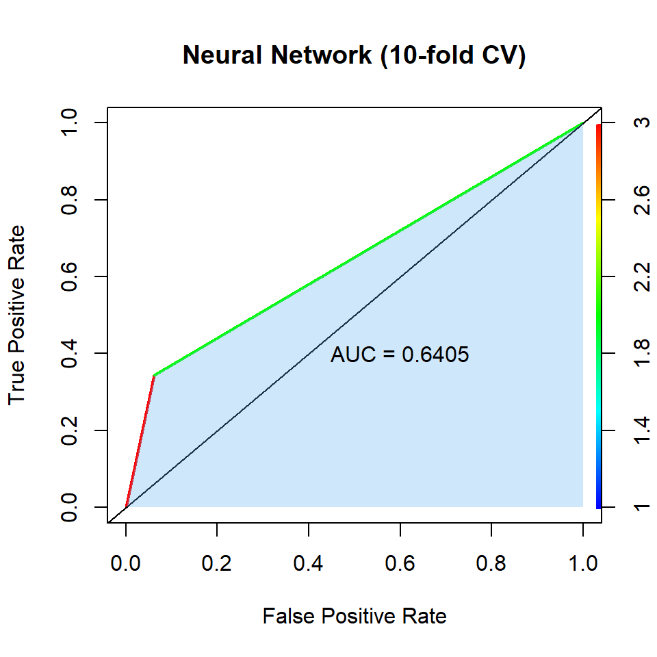
--- title: "Neural Network" --- ```{r setup, include=FALSE} :: opts_chunk$ set (fig.align = TRUE )library (tidyverse) # Load core packages: # ggplot2, for data visualization. # dplyr, for data manipulation. # tidyr, for data tidying. # purrr, for functional programming. # tibble, for tibbles, a modern re-imagining of data frames. # stringr, for strings. # forcats, for factors. # lubridate, for date/times. # readr, for reading .csv, .tsv, and .fwf files. # readxl, for reading .xls, and .xlxs files. # feather, for sharing with Python and other languages. # haven, for SPSS, SAS and Stata files. # httr, for web apis. # jsonlite for JSON. # rvest, for web scraping. # xml2, for XML. # modelr, for modelling within a pipeline # broom, for turning models into tidy data # hms, for times. library (magrittr) # Pipeline operator library (lobstr) # Visualizing abstract syntax trees, stack trees, and object sizes library (pander) # Exporting/converting complex pandoc documents, EX: df to Pandoc table library (ggforce) # More plot functions on top of ggplot2 library (ggpubr) # Automatically add p-values and significance levels plots. # Arrange and annotate multiple plots on the same page. # Change graphical parameters such as colors and labels. library (sf) # Geo-spatial vector manipulation: points, lines, polygons library (kableExtra) # Generate 90 % of complex/advanced/self-customized/beautiful tables library (cowplot) # Multiple plots arrangement library (gridExtra) # Multiple plots arrangement library (animation) # Animated figure container library (latex2exp) # Latex axis titles in ggplot2 library (ellipse) # Simultaneous confidence interval region to check C.I. of 2 slope parameters library (plotly) # User interactive plots library (ellipse) # Simultaneous confidence interval region to check C.I. of 2 regressors library (olsrr) # Model selections library (leaps) # Regression subsetting library (pls) # Partial Least squares library (MASS) # LDA, QDA, OLS, Ridge Regression, Box-Cox, stepAIC, etc,. library (e1071) # Naive Bayesian Classfier, SVM, GKNN, ICA, LCA library (class) # KNN, SOM, LVQ library (ROCR) # Precision/Recall/Sensitivity/Specificity performance plot library (boot) # LOOCV, Bootstrap, library (caret) # Classification/Regression Training, run ?caret::trainControl library (corrgram) # for correlation matrix library (corrplot) # for graphical display of correlation matrix set.seed (1234 ) # make random results reproducible <- getwd ()if (! is.null (current_dir)) {setwd (current_dir)remove (current_dir)``` ## Model Construction ```{r nnet.model_savings, eval=FALSE} #-------------# #----NNet-----# #-------------# set.seed (1234 )<- trainControl (method = "cv" , number = 10 )set.seed (1234 )<- train (good ~ ., data = train, method = "nnet" , trControl = train_control)save (nnet_model, file = "dataset \\ model \\ nnet.model_kfoldCV.Rdata" )``` ## K-fold CV ```{r nnet.kfoldCV, fig.show='hide'} # Data Import load ("dataset \\ wine.data_cleaned.Rdata" )load ("dataset \\ train.Rdata" )load ("dataset \\ test.Rdata" )# Function Import load ("dataset \\ function \\ accu.kappa.plot.Rdata" )# Model import load ("dataset \\ model \\ nnet.model_kfoldCV.Rdata" )<- predict (nnet_model, newdata = test)confusionMatrix (nnet.predictions, test$ good)<- as.numeric (nnet.predictions)<- prediction (nnet.predictions, test$ good)<- performance (pred_obj, "auc" )@ y.values[[1 ]]<- performance (pred_obj, "tpr" , "fpr" )plot (roc_obj, colorize = TRUE , lwd = 2 ,xlab = "False Positive Rate" , ylab = "True Positive Rate" ,main = "Neural Network (10-fold CV)" )abline (a = 0 , b = 1 )<- as.numeric (unlist (roc_obj@ x.values))<- as.numeric (unlist (roc_obj@ y.values))polygon (x = x_values, y = y_values, col = rgb (0.3803922 , 0.6862745 , 0.9372549 , alpha = 0.3 ),border = NA )polygon (x = c (0 , 1 , 1 ), y = c (0 , 0 , 1 ), col = rgb (0.3803922 , 0.6862745 , 0.9372549 , alpha = 0.3 ),border = NA )text (0.6 , 0.4 , paste ("AUC =" , round (auc_val, 4 )))<- recordPlot ():: pander (nnet_model$ results)``` ## Summary ```{r fig.width=5, fig.height=5} :: plot_grid (nnet.kfoldCV.ROC.plot)``` ```{r, echo=FALSE} save (nnet.kfoldCV.ROC.plot, file = "dataset \\ plot \\ nnet.kfoldCV.ROC.plot.Rdata" )```