The CART (Classification and Regression Trees) algorithm is a decision tree method. CART is a popular algorithm used for both classification and regression problems. For our classification task, it constructs a binary tree in which each internal node represents a test on a single feature, and each leaf node represents a class label or a numeric value. The splitting of nodes in the tree is based on a measure of impurity such as Gini impurity or entropy. The CART algorithm is often used in applications such as finance, marketing, and healthcare.
Model Construction
Show/Hide Code
#----------------------##----Decision Tree-----##----------------------#set.seed(1234)train_control <-trainControl(method ="cv", number =10)set.seed(1234)dc_model <-train(good ~ ., data = train, method ="rpart2", trControl = train_control,na.action = na.omit)save(dc_model, file ="dataset\\model\\dc.model_kfoldCV.Rdata")#----------------------------##----Decision Tree (Mod)-----##----------------------------#set.seed(1234)train_control <-trainControl(method ="cv", number =10)set.seed(1234)dc_model <-train(good ~ ., data = train, method ="rpart", trControl = train_control,tuneLength =5,tuneGrid =data.frame(cp =seq(0.001, 0.1, by =0.005)))save(dc_model, file ="dataset\\model\\dc.model_kfoldCV_mod.Rdata")
K-fold CV
Show/Hide Code
# Data Importload("dataset\\wine.data_cleaned.Rdata")load("dataset\\train.Rdata")load("dataset\\test.Rdata")# Function Importload("dataset\\function\\accu.kappa.plot.Rdata")# Model importload("dataset\\model\\dc.model_kfoldCV.Rdata")dc.predictions <-predict(dc_model, newdata = test)confusionMatrix(dc.predictions, test$good)
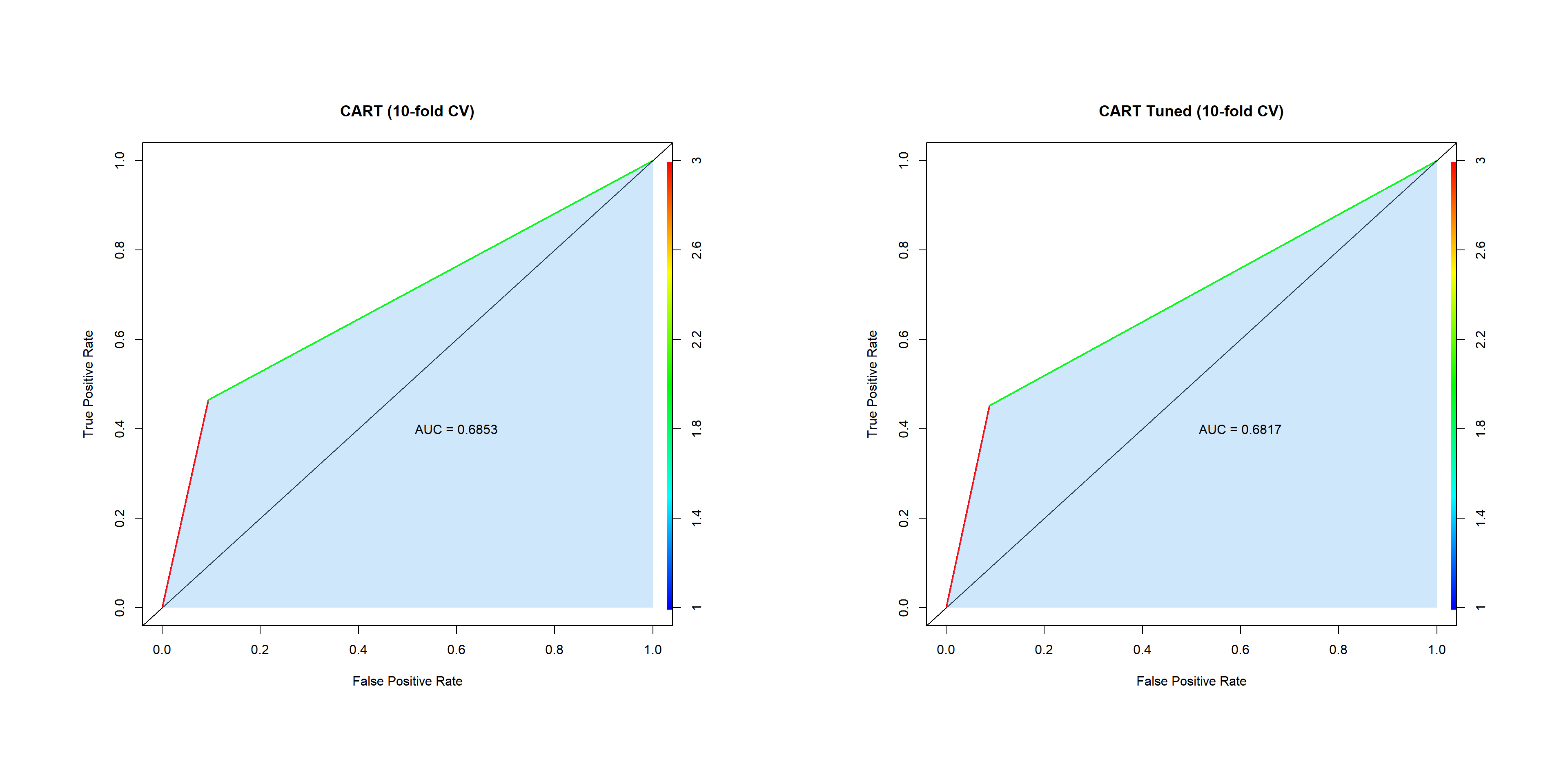
Confusion Matrix and Statistics

          Reference
Prediction   0   1
         0 860 128
         1  89 111

               Accuracy : 0.8173
                 95% CI : (0.7942, 0.8389)
    No Information Rate : 0.7988
    P-Value [Acc > NIR] : 0.058574

                  Kappa : 0.3947

 Mcnemar's Test P-Value : 0.009891

            Sensitivity : 0.9062
            Specificity : 0.4644
         Pos Pred Value : 0.8704
         Neg Pred Value : 0.5550
             Prevalence : 0.7988
         Detection Rate : 0.7239
   Detection Prevalence : 0.8316
      Balanced Accuracy : 0.6853

       'Positive' Class : 0
---title: "Decision Tree"---```{r setup, include=FALSE}knitr::opts_chunk$set(fig.align =TRUE)library(tidyverse) # Load core packages: # ggplot2, for data visualization.# dplyr, for data manipulation.# tidyr, for data tidying.# purrr, for functional programming.# tibble, for tibbles, a modern re-imagining of data frames.# stringr, for strings.# forcats, for factors.# lubridate, for date/times.# readr, for reading .csv, .tsv, and .fwf files.# readxl, for reading .xls, and .xlxs files.# feather, for sharing with Python and other languages.# haven, for SPSS, SAS and Stata files.# httr, for web apis.# jsonlite for JSON.# rvest, for web scraping.# xml2, for XML.# modelr, for modelling within a pipeline# broom, for turning models into tidy data# hms, for times.library(magrittr) # Pipeline operatorlibrary(lobstr) # Visualizing abstract syntax trees, stack trees, and object sizeslibrary(pander) # Exporting/converting complex pandoc documents, EX: df to Pandoc tablelibrary(ggforce) # More plot functions on top of ggplot2library(ggpubr) # Automatically add p-values and significance levels plots. # Arrange and annotate multiple plots on the same page. # Change graphical parameters such as colors and labels.library(sf) # Geo-spatial vector manipulation: points, lines, polygonslibrary(kableExtra) # Generate 90 % of complex/advanced/self-customized/beautiful tableslibrary(cowplot) # Multiple plots arrangementlibrary(gridExtra) # Multiple plots arrangementlibrary(animation) # Animated figure containerlibrary(latex2exp) # Latex axis titles in ggplot2library(ellipse) # Simultaneous confidence interval region to check C.I. of 2 slope parameterslibrary(plotly) # User interactive plotslibrary(ellipse) # Simultaneous confidence interval region to check C.I. of 2 regressorslibrary(olsrr) # Model selections library(leaps) # Regression subsetting library(pls) # Partial Least squareslibrary(MASS) # LDA, QDA, OLS, Ridge Regression, Box-Cox, stepAIC, etc,.library(e1071) # Naive Bayesian Classfier,SVM, GKNN, ICA, LCAlibrary(class) # KNN, SOM, LVQlibrary(ROCR) # Precision/Recall/Sensitivity/Specificity performance plot library(boot) # LOOCV, Bootstrap,library(caret) # Classification/Regression Training, run ?caret::trainControllibrary(corrgram) # for correlation matrixlibrary(corrplot) # for graphical display of correlation matrixset.seed(1234) # make random results reproduciblecurrent_dir <-getwd()if (!is.null(current_dir)) {setwd(current_dir)remove(current_dir)}```The CART (Classification and Regression Trees) algorithm is a decision tree method. CART is a popular algorithm used for both classification and regression problems. For our classification task, it constructs a binary tree in which each internal node represents a test on a single feature, and each leaf node represents a class label or a numeric value. The splitting of nodes in the tree is based on a measure of impurity such as Gini impurity or entropy. The CART algorithm is often used in applications such as finance, marketing, and healthcare.## Model Construction```{r nb.model_savings, eval=FALSE}#----------------------##----Decision Tree-----##----------------------#set.seed(1234)train_control <-trainControl(method ="cv", number =10)set.seed(1234)dc_model <-train(good ~ ., data = train, method ="rpart2", trControl = train_control,na.action = na.omit)save(dc_model, file ="dataset\\model\\dc.model_kfoldCV.Rdata")#----------------------------##----Decision Tree (Mod)-----##----------------------------#set.seed(1234)train_control <-trainControl(method ="cv", number =10)set.seed(1234)dc_model <-train(good ~ ., data = train, method ="rpart", trControl = train_control,tuneLength =5,tuneGrid =data.frame(cp =seq(0.001, 0.1, by =0.005)))save(dc_model, file ="dataset\\model\\dc.model_kfoldCV_mod.Rdata")```## K-fold CV```{r dc.kfoldCV, fig.show='hide'}# Data Importload("dataset\\wine.data_cleaned.Rdata")load("dataset\\train.Rdata")load("dataset\\test.Rdata")# Function Importload("dataset\\function\\accu.kappa.plot.Rdata")# Model importload("dataset\\model\\dc.model_kfoldCV.Rdata")dc.predictions <-predict(dc_model, newdata = test)confusionMatrix(dc.predictions, test$good)dc.predictions <-as.numeric(dc.predictions)pred_obj <-prediction(dc.predictions, test$good)auc_val <-performance(pred_obj, "auc")@y.values[[1]]auc_valroc_obj <-performance(pred_obj, "tpr", "fpr")plot(roc_obj, colorize =TRUE, lwd =2,xlab ="False Positive Rate", ylab ="True Positive Rate",main ="CART (10-fold CV)")abline(a =0, b =1)x_values <-as.numeric(unlist(roc_obj@x.values))y_values <-as.numeric(unlist(roc_obj@y.values))polygon(x = x_values, y = y_values, col =rgb(0.3803922, 0.6862745, 0.9372549, alpha =0.3),border =NA)polygon(x =c(0, 1, 1), y =c(0, 0, 1), col =rgb(0.3803922, 0.6862745, 0.9372549, alpha =0.3),border =NA)text(0.6, 0.4, paste("AUC =", round(auc_val, 4)))dc.kfoldCV.ROC.plot <-recordPlot()dc_df <-data.frame(k= dc_model$results$maxdepth,Accuracy=dc_model$results$Accuracy,Kappa=dc_model$results$Kappa)dc.kfoldCV.plot <-accu.kappa.plot(dc_df) +geom_text(aes(x = k, y = Accuracy, label =round(Accuracy, 3)), hjust =-0.3, angle=90) +geom_text(aes(x = k, y = Kappa, label =round(Kappa, 3)), hjust =-0.3, angle=90) +labs(x="Max Depth")ggtitle("CART Model Performance")pander::pander(dc_model$results)```### Tuned```{r, dc.kfoldCV_mod, fig.show='hide'}# Model Importload("dataset\\model\\dc.model_kfoldCV_mod.Rdata")dc.predictions <-predict(dc_model, newdata = test)confusionMatrix(dc.predictions, test$good)dc.predictions <-as.numeric(dc.predictions)pred_obj <-prediction(dc.predictions, test$good)auc_val <-performance(pred_obj, "auc")@y.values[[1]]auc_valroc_obj <-performance(pred_obj, "tpr", "fpr")plot(roc_obj, colorize =TRUE, lwd =2,xlab ="False Positive Rate", ylab ="True Positive Rate",main ="CART Tuned (10-fold CV)")abline(a =0, b =1)x_values <-as.numeric(unlist(roc_obj@x.values))y_values <-as.numeric(unlist(roc_obj@y.values))polygon(x = x_values, y = y_values, col =rgb(0.3803922, 0.6862745, 0.9372549, alpha =0.3),border =NA)polygon(x =c(0, 1, 1), y =c(0, 0, 1), col =rgb(0.3803922, 0.6862745, 0.9372549, alpha =0.3),border =NA)text(0.6, 0.4, paste("AUC =", round(auc_val, 4)))dc.kfoldCV_mod.ROC.plot <-recordPlot()pander::pander(dc_model$results)```## Summary```{r fig.width=20, fig.height=10}cowplot::plot_grid(dc.kfoldCV.ROC.plot, dc.kfoldCV_mod.ROC.plot, ncol =2, align ="hv", scale =0.8)```| Model | Error Rate | Sensitivity | Specificity | AUC || -------------------- | ---------- | ----------- | ----------- | --------- || CART | 0.1827 | 0.9062 | 0.4644 | 0.6853261 || CART (Tuned) | 0.1810 | 0.9115 | 0.4519 | 0.6816843 |```{r, echo=FALSE}save(dc.kfoldCV.ROC.plot, file ="dataset\\plot\\dc.kfoldCV.ROC.plot.Rdata")save(dc.kfoldCV_mod.ROC.plot, file ="dataset\\plot\\dc.kfoldCV_mod.ROC.plot.Rdata")```