#--------------------##-----K-fold CV------##--------------------#set.seed(1234)# Define the training control object for 10-fold cross-validationtrain_control <-trainControl(method ="cv", number =10)# Train the KNN model using 10-fold cross-validation# tuneLength argument to specify the range of values of K to be considered for tuningset.seed(1234)knn_model <-train(good ~ ., data = train, method ="knn", trControl = train_control,tuneGrid =data.frame(k =1:10))# Save the model into .Rdata for future import save(knn_model, file ="dataset\\knn.model_kfoldCV.Rdata")#--------------------------##-----K-fold CV (Mod)------##--------------------------#set.seed(1234)train_control <-trainControl(method ="cv", number =10)set.seed(1234)knn_model <-train(good ~ ., data = train, method ="knn", trControl = train_control, tuneGrid =data.frame(k =1:30))# Save the model into .Rdata for future import save(knn_model, file ="dataset\\knn.model_kfoldCV_mod.Rdata")#--------------------##----Hold-out CV-----##--------------------#set.seed(1234)train_control <-trainControl(method ="none",)set.seed(1234)knn_model <-train(good ~ ., data = train, method ="knn",tuneGrid =data.frame(k =1:10))save(knn_model, file ="dataset\\knn.model_holdoutCV.Rdata")#--------------------------##----Hold-out CV (Mod)-----##--------------------------#set.seed(1234)train_control <-trainControl(method ="none",)set.seed(1234)knn_model <-train(good ~ ., data = train, method ="knn",tuneGrid =expand.grid(k=1:30))save(knn_model, file ="dataset\\knn.model_holdoutCV_mod.Rdata")#--------------------##-------LOOCV--------##--------------------#set.seed(1234)train_control <-trainControl(method ="LOOCV")set.seed(1234)knn_model <-train(good ~ ., data = train, method ="knn", trControl = train_control,tuneGrid =data.frame(k =1:10))save(knn_model, file ="dataset\\knn.model_looCV.Rdata")#--------------------------##-------LOOCV (Mod)--------##--------------------------#set.seed(1234)train_control <-trainControl(method ="LOOCV")set.seed(1234)knn_model <-train(good ~ ., data = train, method ="knn", trControl = train_control,tuneLength =10,tuneGrid =expand.grid(k =1:20))save(knn_model, file ="dataset\\knn.model_looCV_mod.Rdata")#--------------------##----Repeated CV-----##--------------------#set.seed(1234)train_control <-trainControl(method ="repeatedcv", number =10, repeats =5)set.seed(1234)knn_model <-train(good ~ ., data = train, method ="knn", trControl = train_control)save(knn_model, file ="dataset\\knn.model_repeatedCV.Rdata")#--------------------------##----Repeated CV (Mod)-----##--------------------------#set.seed(1234)train_control <-trainControl(method ="repeatedcv", number =10, repeats =5)kknn.grid <-expand.grid(kmax =c(3, 5, 7 ,9, 11), distance =c(1, 2, 3),kernel =c("rectangular", "gaussian", "cos"))set.seed(1234)knn_model <-train(good ~ ., data = train, method ="kknn",trControl = train_control, tuneGrid = kknn.grid,preProcess =c("center", "scale"))save(knn_model, file ="dataset\\knn.model_repeatedCV_mod.Rdata")
K-fold CV
Show/Hide Code
# Data Importload("dataset\\train.Rdata")load("dataset\\test.Rdata")# Model Importload("dataset\\model\\knn.model_kfoldCV.Rdata")# Make predictions on the test data using the trained model and calculate the test error rateknn.predictions <-predict(knn_model, newdata = test)confusionMatrix(knn.predictions, test$good)
Confusion Matrix and Statistics

          Reference
Prediction   0   1
         0 908 168
         1  41  71

               Accuracy : 0.8241
                 95% CI : (0.8012, 0.8453)
    No Information Rate : 0.7988
    P-Value [Acc > NIR] : 0.01529

                  Kappa : 0.3169

 Mcnemar's Test P-Value : < 2e-16

            Sensitivity : 0.9568
            Specificity : 0.2971
         Pos Pred Value : 0.8439
         Neg Pred Value : 0.6339
             Prevalence : 0.7988
         Detection Rate : 0.7643
   Detection Prevalence : 0.9057
      Balanced Accuracy : 0.6269

       'Positive' Class : 0
Show/Hide Code
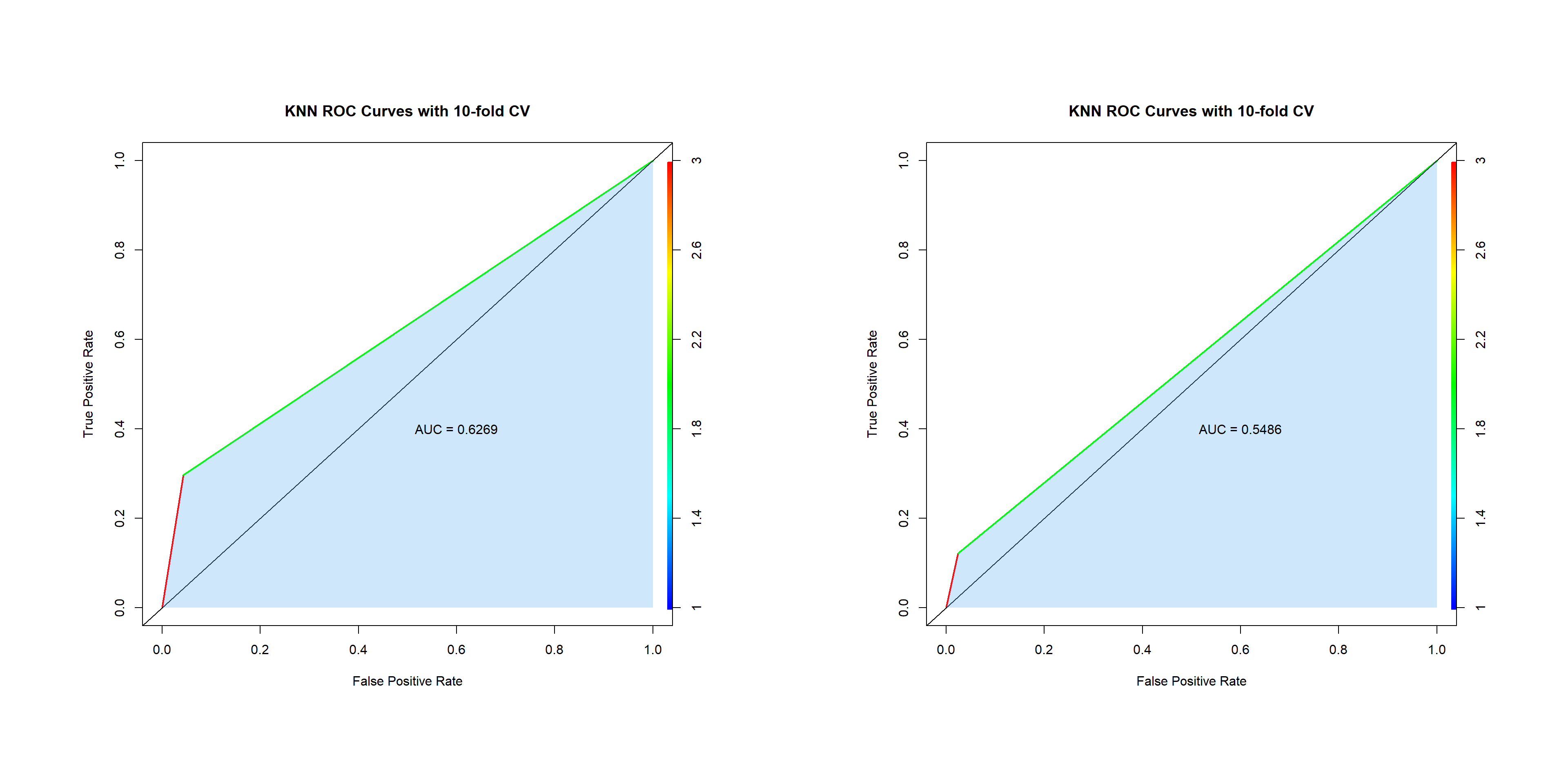
# Convert predictions to a numeric vectorknn.predictions <-as.numeric(knn.predictions)# Calculate the AUC using the performance() and auc() functions:pred_obj <-prediction(knn.predictions, test$good)auc_val <-performance(pred_obj, "auc")@y.values[[1]]auc_val
[1] 0.6269339
Show/Hide Code
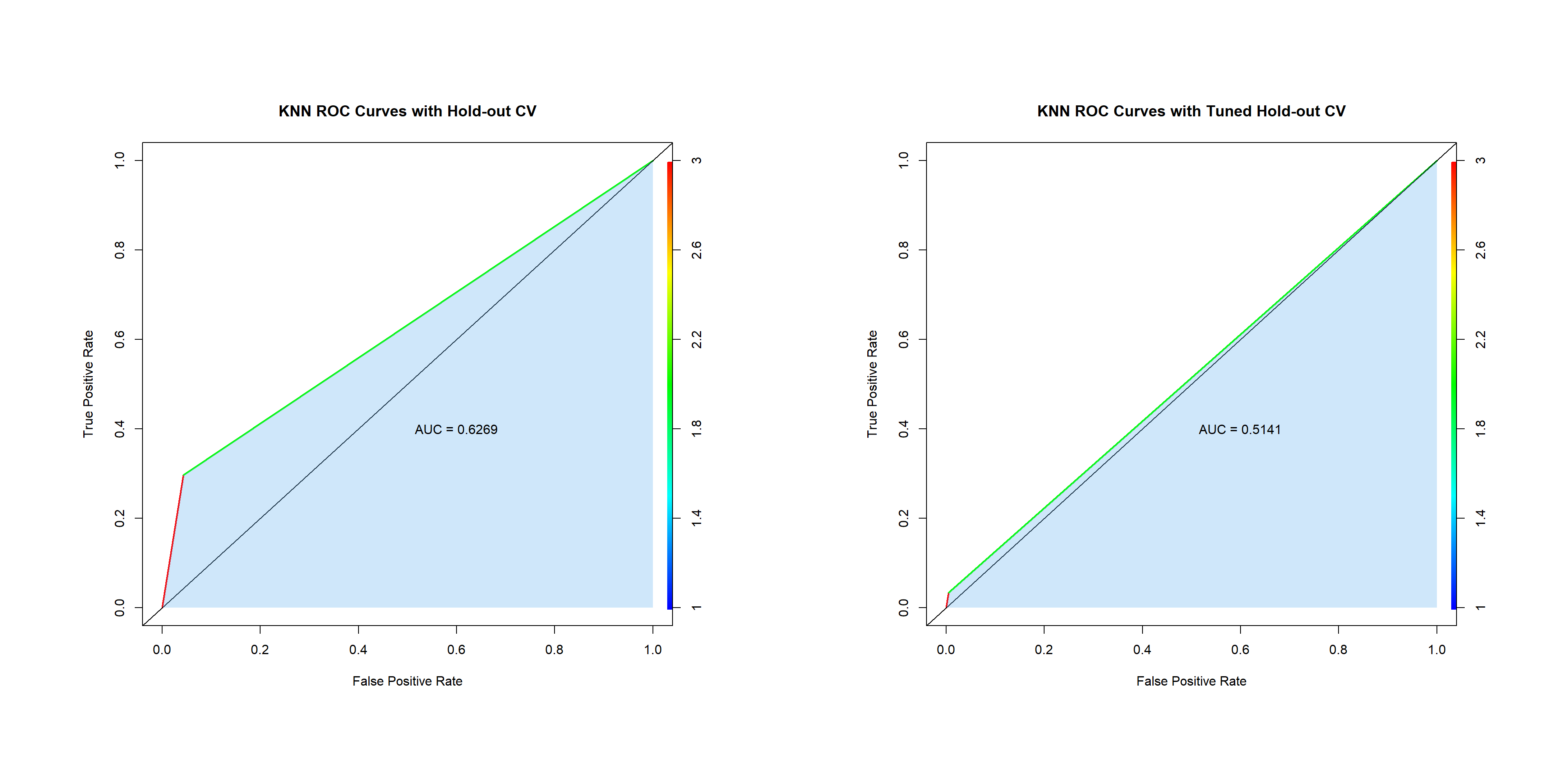
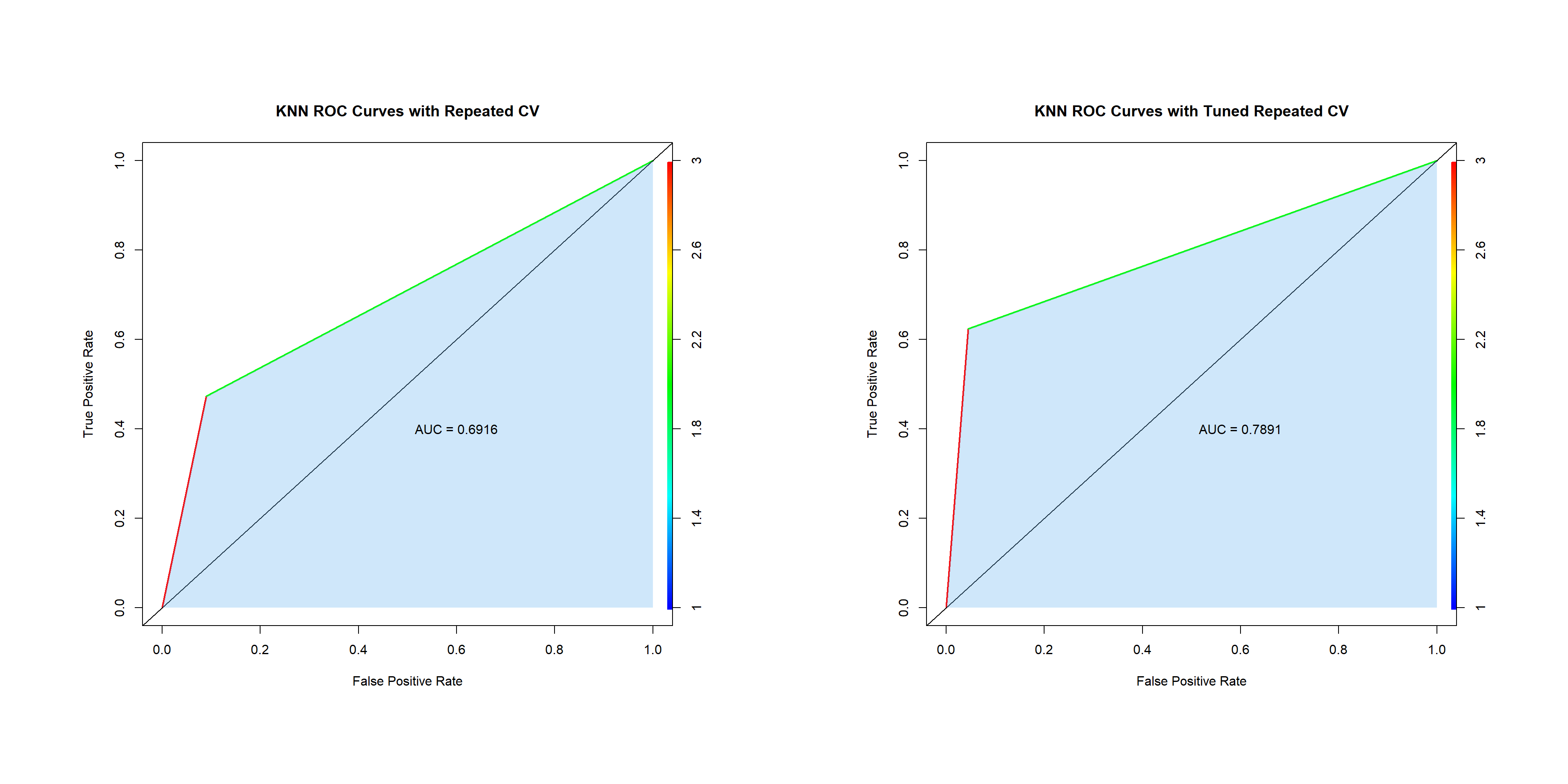
# Performance plot for TP and FProc_obj <-performance(pred_obj, "tpr", "fpr")plot(roc_obj, colorize =TRUE, lwd =2,xlab ="False Positive Rate", ylab ="True Positive Rate",main ="KNN ROC Curves with 10-fold CV")abline(a =0, b =1)x_values <-as.numeric(unlist(roc_obj@x.values))y_values <-as.numeric(unlist(roc_obj@y.values))polygon(x = x_values, y = y_values, col =rgb(0.3803922, 0.6862745, 0.9372549, alpha =0.3),border =NA)polygon(x =c(0, 1, 1), y =c(0, 0, 1), col =rgb(0.3803922, 0.6862745, 0.9372549, alpha =0.3),border =NA)text(0.6, 0.4, paste("AUC =", round(auc_val, 4)))
Show/Hide Code
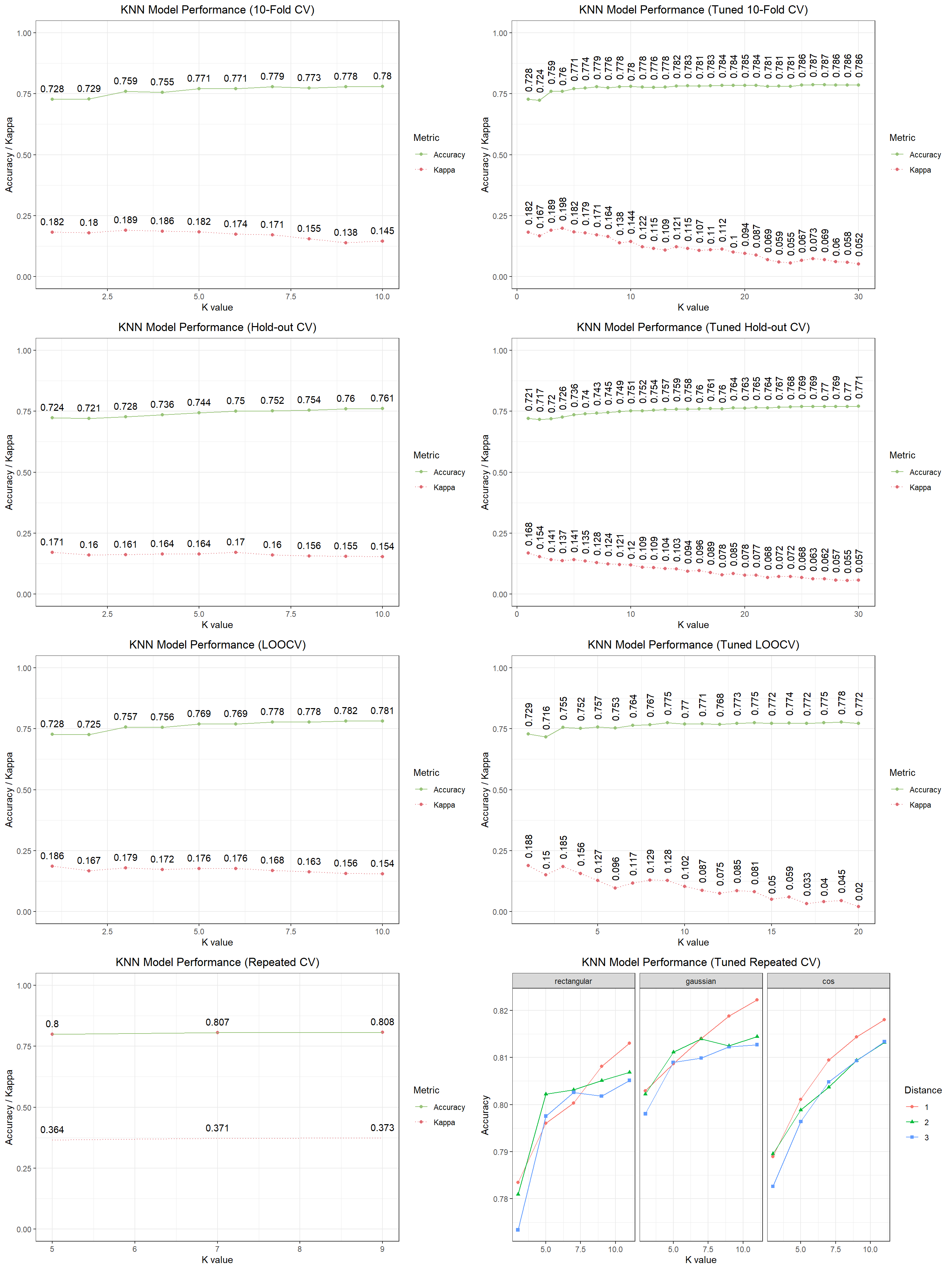
knn.kfoldCV.ROC.plot<-recordPlot()knn_df <-data.frame(k = knn_model$results$k, Accuracy = knn_model$results$Accuracy,Kappa = knn_model$results$Kappa)# Accuracy and Kappa value plotaccu.kappa.plot <-function(model_df) { p <-ggplot(data = model_df) +geom_point(aes(x = k, y = Accuracy, color ="Accuracy")) +geom_point(aes(x = k, y = Kappa, color ="Kappa")) +geom_line(aes(x = k, y = Accuracy, linetype ="Accuracy", color ="Accuracy")) +geom_line(aes(x = k, y = Kappa, linetype ="Kappa", color ="Kappa")) +scale_color_manual(values =c("#98c379", "#e06c75"),guide =guide_legend(override.aes =list(linetype =c(1, 0)) )) +scale_linetype_manual(values=c("solid", "dotted"),guide =guide_legend(override.aes =list(color =c("#98c379", "#e06c75")))) +labs(x ="K value", y ="Accuracy / Kappa") +ylim(0, 1) +theme_bw() +theme(plot.title =element_text(hjust =0.5)) +guides(color =guide_legend(title ="Metric"),linetype =guide_legend(title ="Metric"))return(p)}knn.kfoldCV.plot <-accu.kappa.plot(knn_df) +geom_text(aes(x = k, y = Accuracy, label =round(Accuracy, 3)), vjust =-1) +geom_text(aes(x = k, y = Kappa, label =round(Kappa, 3)), vjust =-1) +ggtitle("KNN Model Performance (10-Fold CV)")