K-fold CV (caret)

Show/Hide Code
#---------------------------#
#----Model Construction-----#
#---------------------------#
set.seed(1234)
# Define the training control object for 10-fold cross-validation
train_control <- trainControl(method = "cv", number = 10)

# Train the logistic regression model using 10-fold cross-validation
set.seed(1234)
logit_model <- train(good ~ ., 
                     data = train, 
                     method = "glm", 
                     family = "binomial",
                     trControl = train_control)

save(logit_model, file = "dataset\\logit.model_kfoldCV.Rdata")
Show/Hide Code
# Data Import
load("dataset\\wine.data_cleaned.Rdata")
load("dataset\\train.Rdata")
load("dataset\\test.Rdata")

# Function Import
load("dataset\\function\\accu.kappa.plot.Rdata")

# Model Import
load("dataset\\model\\logit.model_kfoldCV.Rdata")

logit.predictions <- predict(logit_model, newdata = test)

confusionMatrix(logit.predictions, test$good)
Confusion Matrix and Statistics

          Reference
Prediction   0   1
         0 886 163
         1  63  76
                                          
               Accuracy : 0.8098          
                 95% CI : (0.7863, 0.8317)
    No Information Rate : 0.7988          
    P-Value [Acc > NIR] : 0.1832          
                                          
                  Kappa : 0.2983          
                                          
 Mcnemar's Test P-Value : 4.537e-11       
                                          
            Sensitivity : 0.9336          
            Specificity : 0.3180          
         Pos Pred Value : 0.8446          
         Neg Pred Value : 0.5468          
             Prevalence : 0.7988          
         Detection Rate : 0.7458          
   Detection Prevalence : 0.8830          
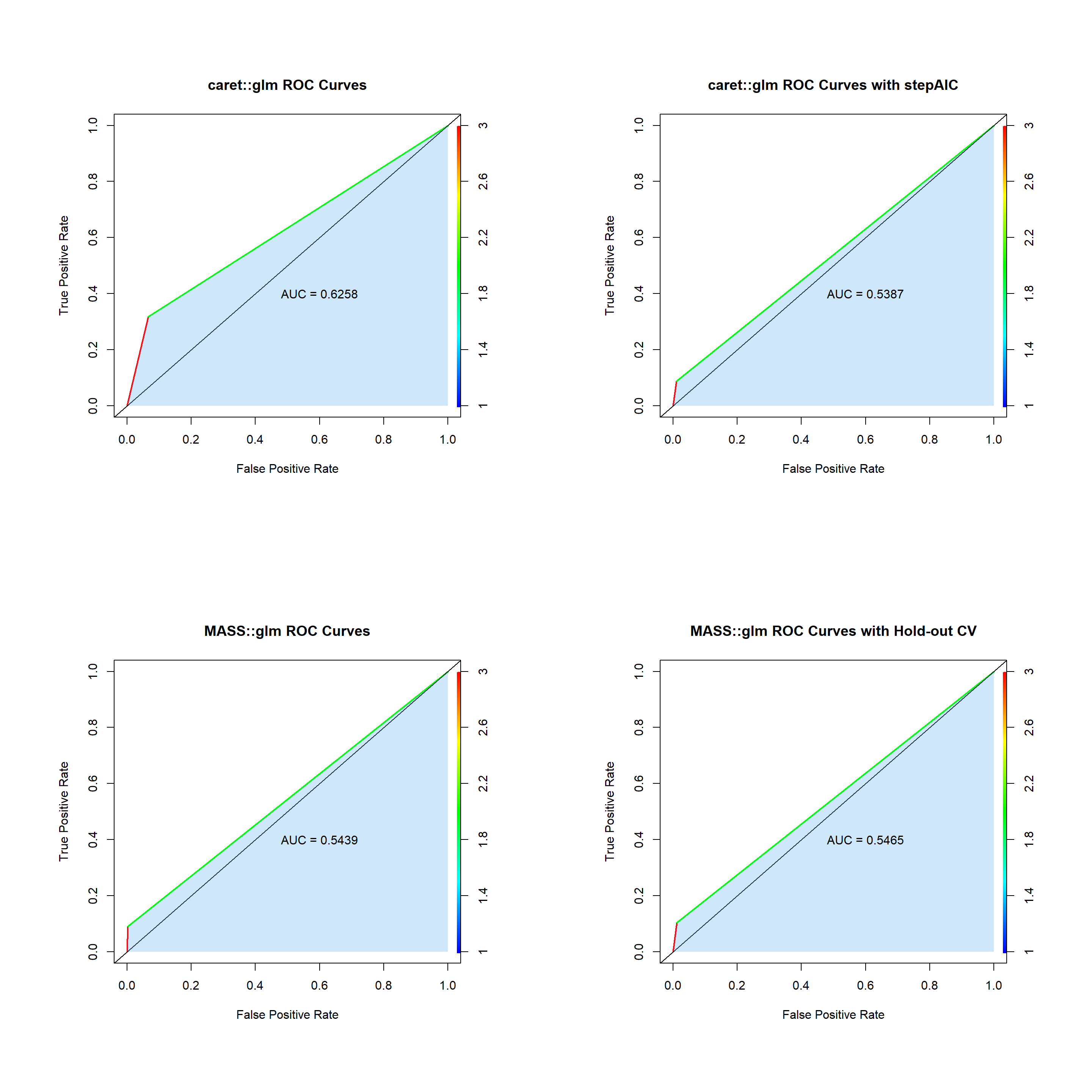
      Balanced Accuracy : 0.6258          
                                          
       'Positive' Class : 0               
                                          
Show/Hide Code
logit.predictions <- as.numeric(logit.predictions)
pred_obj <- prediction(logit.predictions, test$good)

# Compute AUC value
auc_val  <- performance(pred_obj, "auc")@y.values[[1]]
auc_val
[1] 0.625803
Show/Hide Code
log.perf <- performance(pred_obj, "tpr", "fpr")
plot(log.perf, colorize = TRUE, lwd = 2,
     xlab = "False Positive Rate", 
     ylab = "True Positive Rate",
     main = "caret::glm ROC Curves")
abline(a = 0, b = 1)
x_values <- as.numeric(unlist(log.perf@x.values))
y_values <- as.numeric(unlist(log.perf@y.values))
polygon(x = x_values, y = y_values, 
        col = rgb(0.3803922, 0.6862745, 0.9372549, alpha = 0.3),
        border = NA)
polygon(x = c(0, 1, 1), y = c(0, 0, 1), 
        col = rgb(0.3803922, 0.6862745, 0.9372549, alpha = 0.3),
        border = NA)
text(0.6, 0.4, paste("AUC =", round(auc_val, 4)))
Show/Hide Code
logit.kfoldCV_caret.ROC.plot <- recordPlot()

K-fold CV Tuned (caret)

Show/Hide Code
glm.model <- glm(good ~ ., data= train,family="binomial")
glm.fit= stepAIC(glm.model, direction = 'backward')
Start:  AIC=2228.76
good ~ fixed.acidity + volatile.acidity + citric.acid + residual.sugar + 
    chlorides + free.sulfur.dioxide + total.sulfur.dioxide + 
    density + pH + sulphates + alcohol

                       Df Deviance    AIC
- citric.acid           1   2205.4 2227.4
- alcohol               1   2205.7 2227.7
<none>                      2204.8 2228.8
- total.sulfur.dioxide  1   2206.9 2228.9
- chlorides             1   2215.2 2237.2
- free.sulfur.dioxide   1   2216.8 2238.8
- sulphates             1   2224.5 2246.5
- fixed.acidity         1   2230.8 2252.8
- volatile.acidity      1   2231.5 2253.5
- density               1   2236.3 2258.3
- residual.sugar        1   2243.8 2265.8
- pH                    1   2259.9 2281.9

Step:  AIC=2227.37
good ~ fixed.acidity + volatile.acidity + residual.sugar + chlorides + 
    free.sulfur.dioxide + total.sulfur.dioxide + density + pH + 
    sulphates + alcohol

                       Df Deviance    AIC
- alcohol               1   2206.2 2226.2
<none>                      2205.4 2227.4
- total.sulfur.dioxide  1   2207.7 2227.7
- chlorides             1   2215.9 2235.9
- free.sulfur.dioxide   1   2217.4 2237.4
- sulphates             1   2225.0 2245.0
- fixed.acidity         1   2230.8 2250.8
- volatile.acidity      1   2231.7 2251.7
- density               1   2237.6 2257.6
- residual.sugar        1   2244.7 2264.7
- pH                    1   2260.8 2280.8

Step:  AIC=2226.16
good ~ fixed.acidity + volatile.acidity + residual.sugar + chlorides + 
    free.sulfur.dioxide + total.sulfur.dioxide + density + pH + 
    sulphates

                       Df Deviance    AIC
- total.sulfur.dioxide  1   2208.0 2226.0
<none>                      2206.2 2226.2
- chlorides             1   2216.4 2234.4
- free.sulfur.dioxide   1   2217.6 2235.6
- sulphates             1   2231.3 2249.3
- volatile.acidity      1   2231.7 2249.7
- fixed.acidity         1   2272.7 2290.7
- pH                    1   2316.6 2334.6
- residual.sugar        1   2383.1 2401.1
- density               1   2512.7 2530.7

Step:  AIC=2226.01
good ~ fixed.acidity + volatile.acidity + residual.sugar + chlorides + 
    free.sulfur.dioxide + density + pH + sulphates

                      Df Deviance    AIC
<none>                     2208.0 2226.0
- free.sulfur.dioxide  1   2218.1 2234.1
- chlorides            1   2218.6 2234.6
- sulphates            1   2232.6 2248.6
- volatile.acidity     1   2238.0 2254.0
- fixed.acidity        1   2274.6 2290.6
- pH                   1   2317.9 2333.9
- residual.sugar       1   2390.9 2406.9
- density              1   2560.1 2576.1
Show/Hide Code
# Make predictions on test data and construct a confusion matrix
logit.predictions <- predict(glm.fit, newdata = test,type = "response")
logit.predictions <- factor(ifelse(logit.predictions > 0.7, 1, 0),
                            levels = c(0, 1))
confusionMatrix(logit.predictions, test$good)
Confusion Matrix and Statistics

          Reference
Prediction   0   1
         0 939 218
         1  10  21
                                          
               Accuracy : 0.8081          
                 95% CI : (0.7845, 0.8301)
    No Information Rate : 0.7988          
    P-Value [Acc > NIR] : 0.2246          
                                          
                  Kappa : 0.1147          
                                          
 Mcnemar's Test P-Value : <2e-16          
                                          
            Sensitivity : 0.98946         
            Specificity : 0.08787         
         Pos Pred Value : 0.81158         
         Neg Pred Value : 0.67742         
             Prevalence : 0.79882         
         Detection Rate : 0.79040         
   Detection Prevalence : 0.97391         
      Balanced Accuracy : 0.53866         
                                          
       'Positive' Class : 0               
                                          
Show/Hide Code
Accuracy <- confusionMatrix(logit.predictions, test$good)$overall[[1]]
Kappa <- confusionMatrix(logit.predictions, test$good)$overall[[2]] 

logit.predictions <- as.numeric(logit.predictions)
pred_obj <- prediction(logit.predictions, test$good)

# Compute AUC value
auc_val <- performance(pred_obj, "auc")@y.values[[1]]
auc_val
[1] 0.5386644
Show/Hide Code
log.perf <- performance(pred_obj, "tpr", "fpr")
plot(log.perf, colorize = TRUE, lwd = 2,
     xlab = "False Positive Rate", 
     ylab = "True Positive Rate",
     main = "caret::glm ROC Curves with stepAIC")
abline(a = 0, b = 1)
x_values <- as.numeric(unlist(log.perf@x.values))
y_values <- as.numeric(unlist(log.perf@y.values))
polygon(x = x_values, y = y_values, 
        col = rgb(0.3803922, 0.6862745, 0.9372549, alpha = 0.3),
        border = NA)
polygon(x = c(0, 1, 1), y = c(0, 0, 1), 
        col = rgb(0.3803922, 0.6862745, 0.9372549, alpha = 0.3),
        border = NA)
text(0.6, 0.4, paste("AUC =", round(auc_val, 4)))
Show/Hide Code
logit.kfoldCV_caret_tuned.ROC.plot <- recordPlot()

K-fold CV (MASS)

Show/Hide Code
# Set the number of folds
k <- 10

# Randomly assign each row in the data to a fold
set.seed(1234) # for reproducibility
fold_indices <- sample(rep(1:k, length.out = nrow(wine.data_cleaned)))

# Initialize an empty list to store the folds
folds <- vector("list", k)

# Assign each row to a fold
for (i in 1:k) {
  folds[[i]] <- which(fold_indices == i)
}

#To store the error rate of each fold
error_rate <- numeric(k)
kappa <- numeric(k)
confusion_matrices <- vector("list", k)

# Loop through each fold
for (i in 1:k) {
  # Extract the i-th fold as the testing set
  test_indices <- unlist(folds[[i]])
  
  test <- wine.data_cleaned[test_indices, ]
  train <- wine.data_cleaned[-test_indices, ]
  
  # Fit the model on the training set
  logit_model <- glm(good ~ ., data = train, family = binomial)
  
  # Make predictions on the testing set and calculate the error rate
  log.pred <- predict(logit_model, newdata = test, type = "response")
  predicted_classes <- as.numeric(ifelse(log.pred > 0.7, 1, 0))
  
  # Compute MAE
  error_rate[i] <- mean((predicted_classes> 0.7) != test$good)
  
  # Compute confusion matrix
  test$good <- as.factor(test$good)
  predicted_classes <- factor(ifelse(log.pred > 0.7, 1, 0), levels = c(0, 1))
  confusion_matrices[[i]] <- caret::confusionMatrix(predicted_classes, test$good)
  
  # Compute Kappa value
  kappa[i] <- confusion_matrices[[i]]$overall[[2]]
  
  # Print the error rates for each fold
  cat(paste0("Fold ", i, ": ", "OER:", error_rate[i], "\n"))
}
Fold 1: OER:0.198992443324937
Fold 2: OER:0.181818181818182
Fold 3: OER:0.20959595959596
Fold 4: OER:0.247474747474747
Fold 5: OER:0.174242424242424
Fold 6: OER:0.22979797979798
Fold 7: OER:0.184343434343434
Fold 8: OER:0.196969696969697
Fold 9: OER:0.161616161616162
Fold 10: OER:0.179292929292929
Show/Hide Code
best_confmat_index <- which.min(error_rate)
best_confmat_index
[1] 9
Show/Hide Code
confusion_matrices[best_confmat_index]
[[1]]
Confusion Matrix and Statistics

          Reference
Prediction   0   1
         0 326  64
         1   0   6
                                          
               Accuracy : 0.8384          
                 95% CI : (0.7984, 0.8733)
    No Information Rate : 0.8232          
    P-Value [Acc > NIR] : 0.2365          
                                          
                  Kappa : 0.1337          
                                          
 Mcnemar's Test P-Value : 3.407e-15       
                                          
            Sensitivity : 1.00000         
            Specificity : 0.08571         
         Pos Pred Value : 0.83590         
         Neg Pred Value : 1.00000         
             Prevalence : 0.82323         
         Detection Rate : 0.82323         
   Detection Prevalence : 0.98485         
      Balanced Accuracy : 0.54286         
                                          
       'Positive' Class : 0               
                                          
Show/Hide Code
#AUC and Performance Plot
predicted_classes <- as.numeric(predicted_classes)
pred_obj <- prediction(predicted_classes, test$good)
auc_val  <- performance(pred_obj, "auc")@y.values[[1]]
log.perf <- performance(pred_obj,"tpr","fpr")
auc_val  <- performance(pred_obj, "auc")@y.values[[1]]
auc_val
[1] 0.5438871
Show/Hide Code
plot(log.perf, colorize = TRUE, lwd = 2,
     xlab = "False Positive Rate", 
     ylab = "True Positive Rate",
     main = "MASS::glm ROC Curves")
abline(a = 0, b = 1)
x_values <- as.numeric(unlist(log.perf@x.values))
y_values <- as.numeric(unlist(log.perf@y.values))
polygon(x = x_values, y = y_values, 
        col = rgb(0.3803922, 0.6862745, 0.9372549, alpha = 0.3),
        border = NA)
polygon(x = c(0, 1, 1), y = c(0, 0, 1), 
        col = rgb(0.3803922, 0.6862745, 0.9372549, alpha = 0.3),
        border = NA)
text(0.6, 0.4, paste("AUC =", round(auc_val, 4)))
Show/Hide Code
logit.kfoldCV_MASS.ROC.plot <- recordPlot()

logit_df <- data.frame(k = 1:k,
                       Accuracy = 1-error_rate, 
                       Kappa = kappa)

logit.kfoldCV_MASS.plot <- accu.kappa.plot(logit_df) + 
  geom_text(aes(x = k, y = Accuracy, label = round(Accuracy, 3)), vjust = -1) +
  geom_text(aes(x = k, y = Kappa, label = round(Kappa, 3)), vjust = -1) +
  ggtitle("MASS::glm Model Performance (10-Fold CV)")

Hold-out CV (MASS)

Show/Hide Code
# Set the seed for reproducibility
set.seed(1234)

# Proportion of data to use for training
train_prop <- 0.7

# Split the data into training and testing sets
train_indices <- sample(seq_len(nrow(wine.data_cleaned)), size = round(train_prop * nrow(wine.data_cleaned)), replace = FALSE)
train <- wine.data_cleaned[train_indices, ]
test <- wine.data_cleaned[-train_indices, ]

# Fit the model on the training set
logit_model <- glm(good ~ ., data = train, family = binomial)

# Make predictions on the testing set and calculate the error rate
log.pred <- predict(logit_model, newdata = test, type = "response")
predicted_classes <- as.numeric(ifelse(log.pred > 0.7, 1, 0))

# Compute error rate
error_rate <- mean((predicted_classes > 0.7) != test$good)

# Calculate the accuracy of the predictions on the testing set
train$good <- as.numeric(train$good)
test$good <- as.factor(test$good)
predicted_classes <- factor(ifelse(log.pred > 0.7, 1, 0), levels = c(0, 1))
confusionMatrix(predicted_classes, test$good)
Confusion Matrix and Statistics

          Reference
Prediction   0   1
         0 938 214
         1  11  25
                                          
               Accuracy : 0.8106          
                 95% CI : (0.7871, 0.8325)
    No Information Rate : 0.7988          
    P-Value [Acc > NIR] : 0.1643          
                                          
                  Kappa : 0.1363          
                                          
 Mcnemar's Test P-Value : <2e-16          
                                          
            Sensitivity : 0.9884          
            Specificity : 0.1046          
         Pos Pred Value : 0.8142          
         Neg Pred Value : 0.6944          
             Prevalence : 0.7988          
         Detection Rate : 0.7896          
   Detection Prevalence : 0.9697          
      Balanced Accuracy : 0.5465          
                                          
       'Positive' Class : 0               
                                          
Show/Hide Code
kappa <- confusionMatrix(predicted_classes, test$good)$overall[[2]]

#AUC and Performance Plot
predicted_classes <- as.numeric(predicted_classes)
pred_obj <- prediction(predicted_classes, test$good)
log.perf <- performance(pred_obj,"tpr","fpr")
auc_val <- performance(pred_obj, "auc")@y.values[[1]]
auc_val
[1] 0.5465057
Show/Hide Code
plot(log.perf, colorize = TRUE, lwd = 2,
     xlab = "False Positive Rate", 
     ylab = "True Positive Rate",
     main = "MASS::glm ROC Curves with Hold-out CV")
abline(a = 0, b = 1)
x_values <- as.numeric(unlist(log.perf@x.values))
y_values <- as.numeric(unlist(log.perf@y.values))
polygon(x = x_values, y = y_values, 
        col = rgb(0.3803922, 0.6862745, 0.9372549, alpha = 0.3),
        border = NA)
polygon(x = c(0, 1, 1), y = c(0, 0, 1), 
        col = rgb(0.3803922, 0.6862745, 0.9372549, alpha = 0.3),
        border = NA)
text(0.6, 0.4, paste("AUC =", round(auc_val, 4)))
Show/Hide Code
logit.holdoutCV_MASS.ROC.plot <- recordPlot()

pander::pander(data.frame("Accuracy" = 1 - error_rate, 
                          "Kappa" = kappa))
Accuracy Kappa
0.8106 0.1363

Summary

Show/Hide Code
cowplot::plot_grid(logit.kfoldCV_caret.ROC.plot,
                   logit.kfoldCV_caret_tuned.ROC.plot,
                   logit.kfoldCV_MASS.ROC.plot,
                   logit.holdoutCV_MASS.ROC.plot,
                   ncol = 2, align = "hv", scale = 0.8)

Model (Resampling Method) Error Rate Sensitivity Specificity AUC
Logistic Regression (caret 10-fold CV) 0.1902 0.9336 0.3180 0.6258030
Logistic Regression (caret tuned with stepAIC) 0.1919 0.9895 0.0879 0.5386644
Logistic Regression (MASS 10-fold CV) 0.1616 1.0000 0.0857 0.5438871
Logistic Regression (MASS Hold-out CV) 0.1894 0.9884 0.1046 0.5465057